Chapter 7 Gradient Echo Imaging Methods Perry Sprawls, Ph.D.
Link to Book Table of Contents	Chapter Contents Shown Below

Introduction And Overview  

It is possible to produce an echo event by applying a magnetic field gradient without a 180˚ RF pulse to the tissue as in the spin echo methods. There are several imaging methods that use the gradient echo technique to produce the RF signals and these make up the gradient echo family of methods.

            The primary advantage of the gradient echo methods over the spin echo methods is that gradient echo methods perform faster image acquisitions. Gradient echo methods are generally considered to be among the faster imaging methods. They are also used in some of the angiographic applications because gradient echo generally produces bright blood, as we will see in Chapter 12, as well as for functional imaging, as described in Chapter 13. One limitation of the gradient echo methods is they do not produce good T2-weighted images, as will be described later in this chapter. However, by combining the gradient and spin echo methods, this limitation can be overcome.

            At this time we will develop the concept of gradient echo and then consider the specific gradient echo imaging methods and their characteristics.

The Gradient Echo Process  

Transverse magnetization is present only when a sufficient quantity of protons are spinning in-phase in the transverse plane. As we have seen, the decay (relaxation) of transverse magnetization is the result of proton dephasing. We also recall that an RF signal is being produced any time there is transverse magnetization and the intensity of the signal is proportional to the level of magnetization.

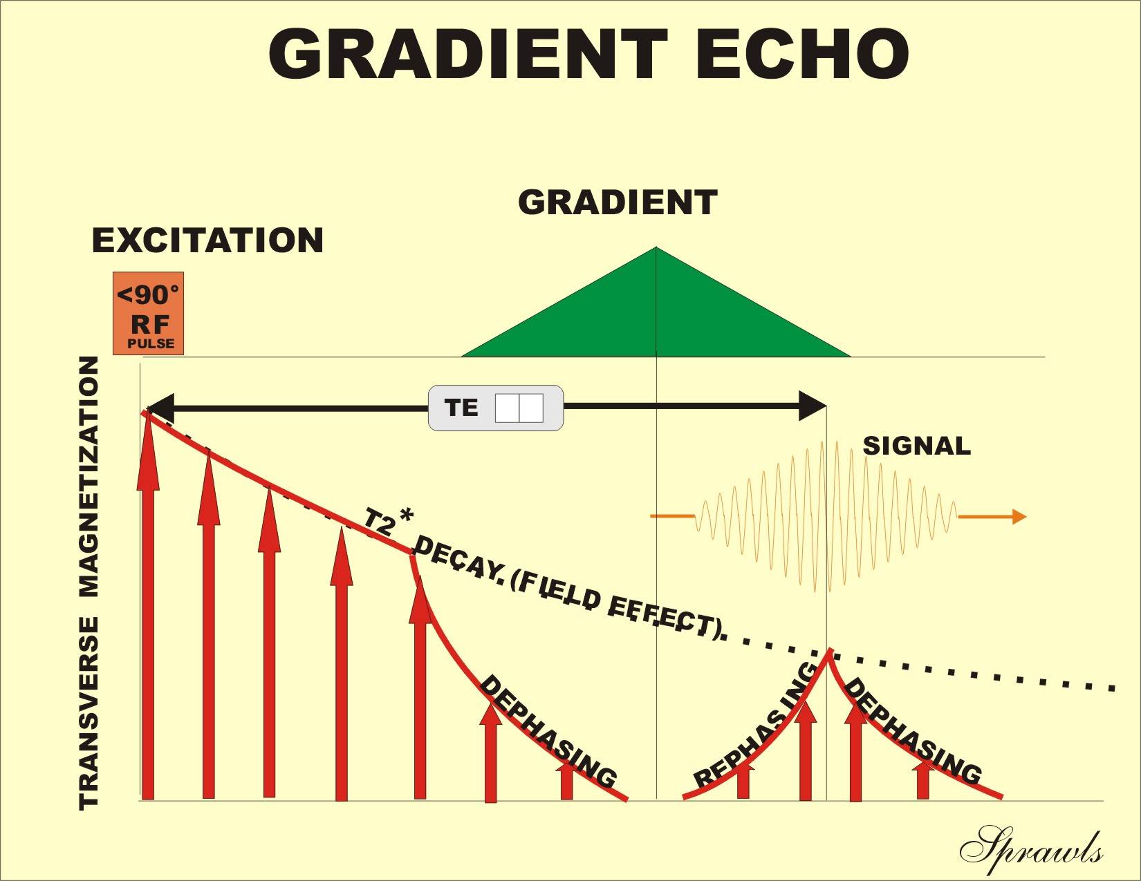
            With the spin echo technique we use an RF pulse to rephase the protons after they have been dephased by inherent magnetic field inhomogeneities and susceptibility effects within the tissue voxel. With the gradient echo technique the protons are first dephased, on purpose, by turning on a gradient and then rephased by reversing the direction of the gradient, as shown in Figure 7-1.

A gradient echo can only be created when transverse magnetization is present. This can be either during the free induction decay (FID) period or during a spin echo event. In Figure 7-1 the gradient echo is being created during the FID. Let us now consider the process in more detail.

            First, transverse magnetization is produced by the excitation pulse. It immediately begins to decay (the FID process) because of the magnetic field inhomogeneities within each individual voxel. The rate of decay is related to the value of T2*. A short time after the excitation pulse a gradient is applied, which produces a very rapid dephasing of the protons and reduction in the transverse magnetization. This occurs because a gradient is a forced inhomogeneity in the magnetic field. The next step is to reverse the direction of the applied gradient. Even though this is still an inhomogeneity in the magnetic field, it is in the opposite direction. This then causes the protons to rephase and produce an echo event. As the protons rephase, the transverse magnetization will reappear and rise to a value determined by the FID process. The gradient echo event is a rather well-defined peak in the transverse magnetization and this, in turn, produces a discrete RF signal.

            The TE is determined by adjusting the time interval between the excitation pulse and the gradients that produce the echo event. TE values for gradient echo are typically much shorter than for spin echo, especially when the gradient echo is produced during the FID.

Small Angle Gradient Echo Methods  

The gradient echo technique is generally used in combination with an RF excitation pulse that has a small flip angle of less than 90˚. We will discover that the advantage of this is that it permits the use of shorter TR values and this, in turn, produces faster image acquisition.

            One source of confusion is that each manufacturer of MRI equipment has given his gradient echo imaging methods different trade names. In this text we will use the generic name of small angle gradient echo (SAGE) method.

            The SAGE method generally requires a shorter acquisition time than the spin echo methods. It is also a more complex method with respect to adjusting contrast sensitivity because the flip angle of the excitation pulse becomes one of the adjustable protocol imaging factors.

Excitation/Saturation-Pulse Flip Angle  

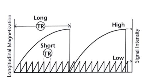
We recall that the purpose of the excitation/ saturation pulse applied at the beginning of an imaging cycle is to convert or flip longitudinal magnetization into transverse magnetization. When a 90° pulse is used, all of the existing longitudinal magnetization is converted into transverse magnetization, as we have seen with the spin echo methods. The 90° pulse reduces the longitudinal magnetization to zero (i.e., complete saturation) at the beginning of each imaging cycle. This then means that a relatively long TR interval must be used to allow the longitudinal magnetization to recover to a useful value. The time required for the longitudinal magnetization to relax or to recover is one of the major factors in determining acquisition time. The effect of reducing TR when 90° pulses are used is shown in Figure 7-2.

 As the TR value is decreased, the longitudinal magnetization grows to a lower value and the amount of transverse magnetization and RF signal intensity produced by each pulse is decreased. The reduced signal intensity results in an increase in image noise as described in Chapter 10. Also, the use of short TR intervals with a 90° pulse (as in spin echo) cannot produce good PD or T2-weighted images.

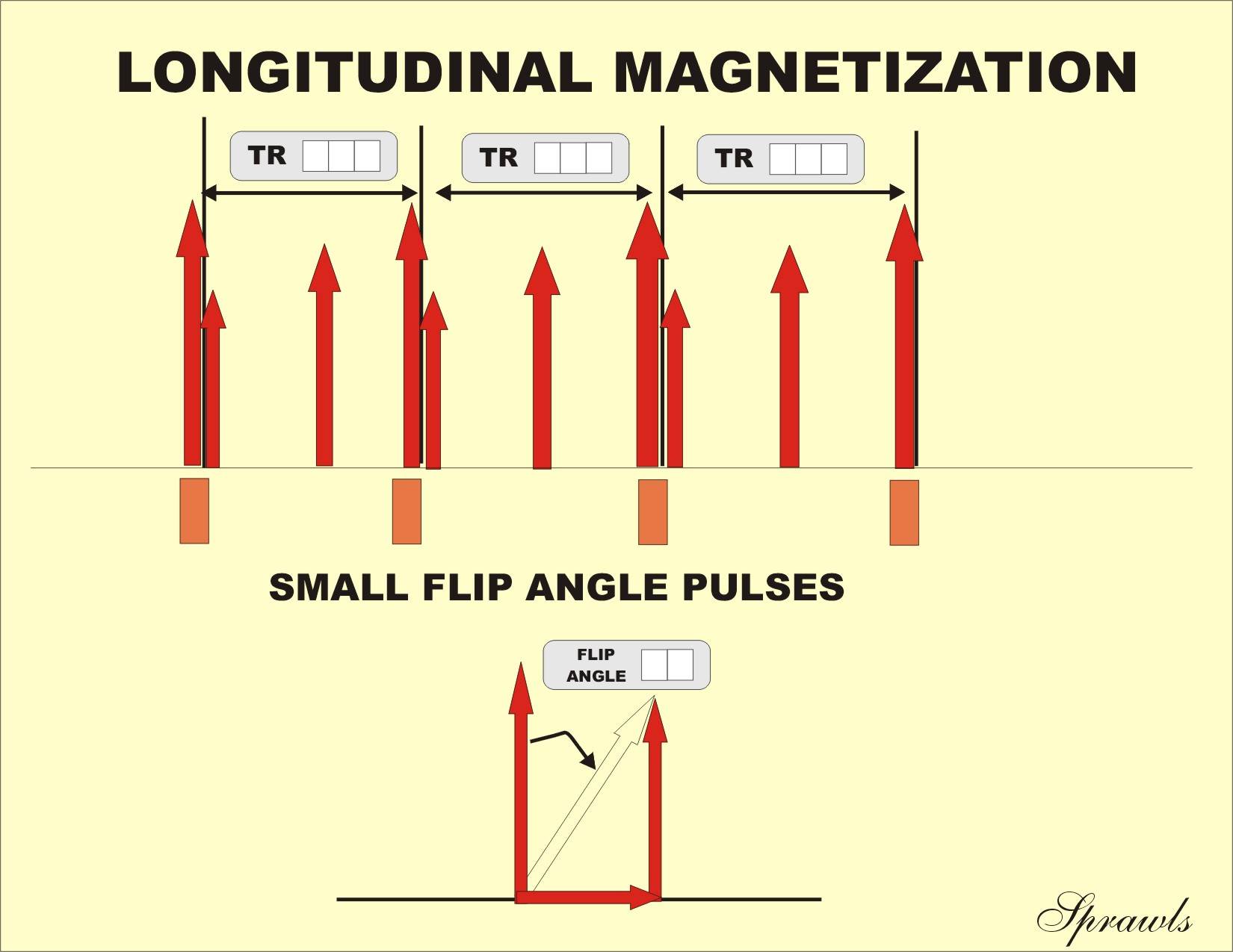
            One approach to reducing TR and increasing acquisition speed without incurring the disadvantages that have just been described is to use a pulse that has a flip angle of less than 90°. A small flip-angle (<90°) pulse converts only a fraction of the longitudinal magnetization into transverse magnetization. This means that the longitudinal magnetization is not completely destroyed or reduced to zero (saturated) by the pulse, as shown in Figure 7-3.

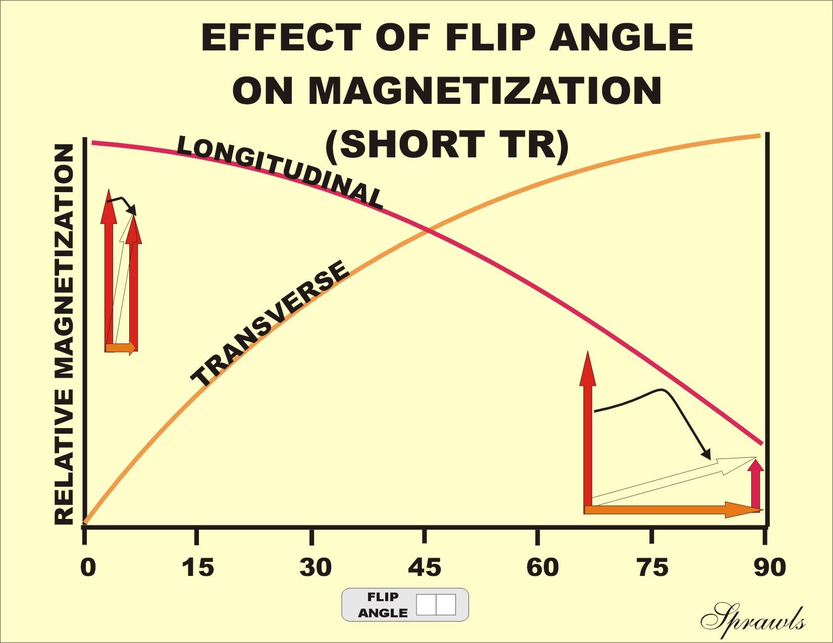
            Reducing the flip angle has two effects that must be considered together. The effect that we have just observed is that the longitudinal magnetization is not completely destroyed and remains at a relatively high level from cycle to cycle, even for short TR intervals. This will increase RF signal intensity compared to the use of 90° pulses. However, as the flip angle is reduced, a smaller fraction of the longitudinal magnetization is converted into transverse magnetization. This has the effect of reducing signal intensity. The result is a combination of these two effects. This is illustrated in Figure 7-4.

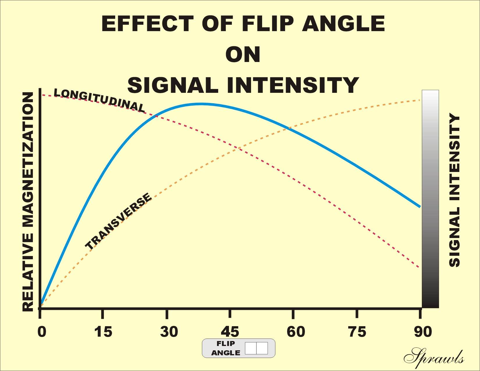
 Here we see that as the flip angle is increased over the range from 0–90°, the level of longitudinal magnetization at the beginning of a cycle decreases. On the other hand, as the angle is increased, the fraction of this longitudinal magnetization that is converted into transverse magnetization increases and RF signal intensity increases. The combination of these two effects is shown in Figure 7-5.

Here we see how changing flip angle affects signal intensity. The exact shape of this curve depends on the specific T1 value of the tissue and the TR interval. For each T1/TR combination there is a different curve and a specific flip angle that produces maximum signal intensity.

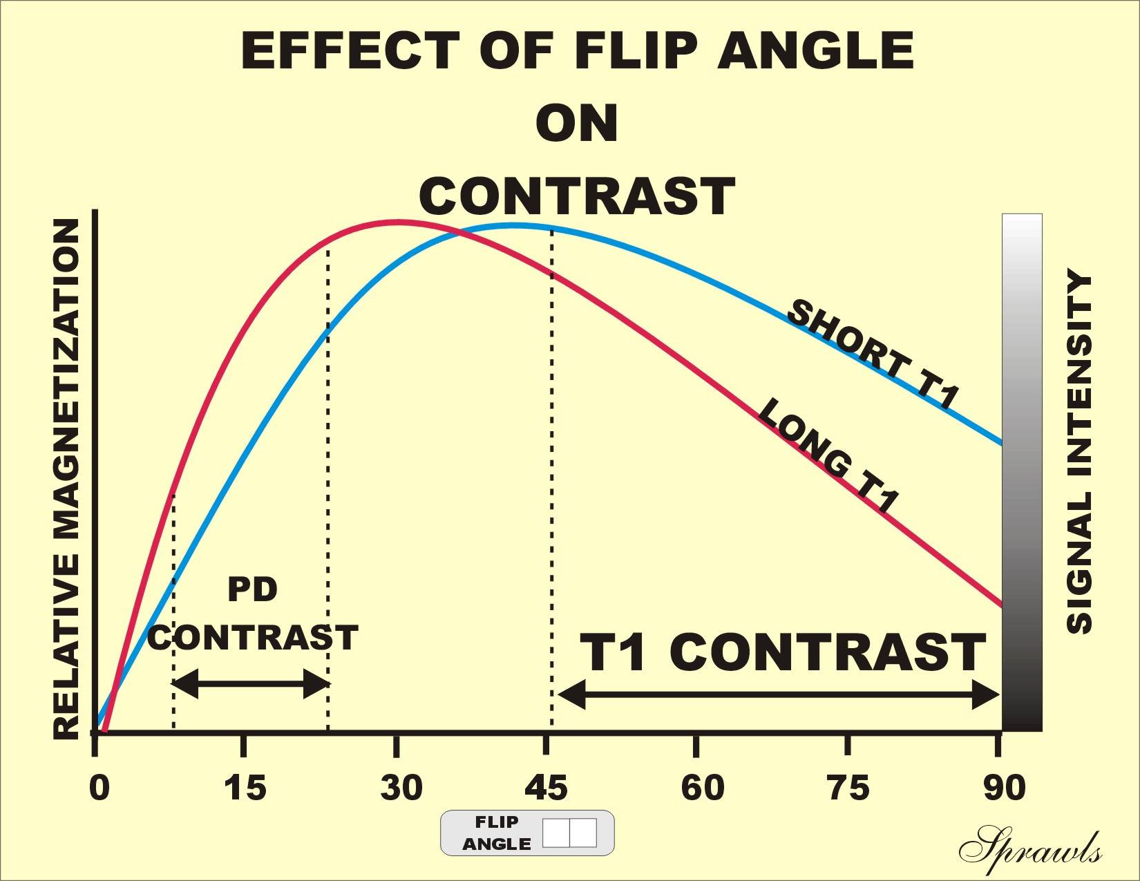
            Let us now use Figure 7-6 to compare the magnetization of two tissues with different T1 values as we change flip angle.

 Contrast between the two tissues is represented by the difference in magnetization levels. At this point we are assuming a short TE and considering the contrast associated with only the longitudinal magnetization. The flip-angle range is divided into several specific segments as shown.

Contrast Sensitivity  

With the SAGE method the contrast sensitivity for a specific tissue characteristic is controlled by three protocol factors. As with spin echo, TR and TE have an effect. However, the flip angle becomes the factor with the greatest effect on contrast. We will now see how changing flip angle can be used to select specific types of contrast with a basic gradient echo method.

T1 Contrast  

Relatively large flip angles (45°–90°) produce T1 contrast. This is what we would expect because large flip angles (close to 90°) and short TR and TE values are similar to the factors used to produce T1 contrast with the spin echo method. Here, with gradient echo, we observe a loss of T1 contrast as the flip angle is decreased significantly from 90°.

Low Contrast  

There is an intermediate range of flip-angle values that produces very little, if any, contrast. This is the region in which the PD and T1 contrast cancel each other for many tissues, such as gray and white matter.

Proton Density (PD) Contrast  

Relatively low flip-angle values produce PD contrast. As the flip angle is reduced within this region, there is a significant decrease in magnetization and the resulting signal intensity.

Up to this point we have observed generally how changing the flip angle of the excitation pulse affects signal intensity and contrast. In the SAGE imaging method the flip angle is one of the imaging factors that must be adjusted by the user. However, it becomes somewhat complex because the specific effect of flip angle is modified by the other imaging factors and techniques used to enhance a specific type of contrast.

T2 and T2* Contrast  

We recall that T2 contrast is produced by the decay characteristics of transverse magnetization and that there are two different decay rates, T2 and T2*. The slower decay rate is determined by the T2 characteristics of the tissue. The faster decay is produced by small inhomogeneities within the magnetic field often related to variations in tissue susceptibility differences. This decay rate is determined by the T2* of the tissue environment. When a spin echo technique is used, the spinning protons are rephased, and the T2* effect is essentially eliminated. However, when a spin echo technique is not used, the transverse magnetization depends on the T2* characteristics. The gradient echo technique does not compensate for the inhomogeneity and susceptibility effect dephasing as the spin echo technique does. Also, without using a spin echo process the long TE values necessary to produce T2 contrast cannot be achieved. Therefore, a basic gradient echo imaging method is not capable of producing true T2 contrast. The contrast will be determined primarily by the T2* characteristics. The amount of T2* contrast in an image is determined by the selected TE value. In general, longer TE values (but short compared to those used in spin echo) produce more T2* contrast.

Contrast Enhancement  

In addition to using combinations of TR, TE, and flip angle to control the contrast characteristics, some gradient echo methods have other features for enhancing certain types of contrast.

            When SAGE methods are used with relatively short TR values, there is the possibility that some of the transverse magnetization created in one imaging cycle will carry over into the next cycle. This happens when the TR values are in the same general range as the T2 values of the tissue. SAGE methods differ in how they use the carry-over transverse magnetization.

            A typical SAGE sequence is limited to one RF pulse per cycle. If additional pulses were used, as in the spin echo techniques, they would affect the longitudinal magnetization and upset its condition of equilibrium. However, because of the relatively short TR values it is possible for the repeating small-angle excitation pulses to produce a spin echo effect. This can occur only when the TR interval is not much longer than the T2 value of the tissue.

            Associated with each excitation pulse, there are actually two components of the transverse magnetization. There is the FID produced by the immediate pulse and a spin echo component produced by the preceding pulses. The spin echo component is related to the T1 characteristics of the tissue. The FID component is related to the T2* characteristics. The contrast characteristics of the imaging method are determined by how these two components are combined. Different combinations are obtained by altering the location of the gradient echo event relative to the transverse magnetization and by turning the spin echo component on or off as described below.

Mixed Contrast  

When both the FID and spin echo components are used, an image with mixed contrast characteristics will be obtained. This method produces a relatively high signal intensity compared to the methods described below.

Spoiling and T1 Contrast Enhancement  

An image with increased Tl contrast is obtained by suppressing the spin echo component. This is known as spoiling. The spin echo component, which is a carryover of transverse magnetization from previous cycles, can be destroyed or spoiled by either altering the phase relationship of the RF pulses or by applying gradient pulses to dephase the spinning protons.

            The basic SAGE method discussed up to this point permits faster (than spin echo) image acquisition because the TR can be set to shorter values. However, the gradient echo process can be used in methods that provide fast acquisition based on an entirely different principle. We will now consider methods that achieve their speed by filling many rows of k space during one acquisition cycle.

            In Chapter 5 we saw that in the acquisition phase the signal data is being directed into k space from which the image will be reconstructed. The k space is filled one row at a time. The number of rows in the k space for a specific image depends on the required image detail. The process that directs the signals into a specific row of k space is the spatial encoding function performed by one of the gradients. This will be described in Chapter 9. In conventional spin echo and SAGE imaging only one row of k space is filled with each imaging cycle. This is because there is only one echo signal produced per cycle that can be encoded to go to a specific row of k space. This means that the size of k space determines the minimum number of cycles that an acquisition must have. We are about to see some gradient echo methods that can fill many rows of k space in one imaging cycle. This is achieved by using the gradient echo process to produce many echo events from the transverse magnetization that is present during one cycle.

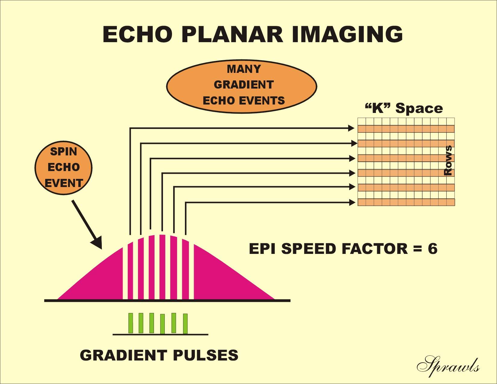
Echo Planar Imaging (EPI) Method  

Echo planar is the fast gradient echo imaging method that is capable of acquiring a complete image in a very short time. However, it requires an MRI system equipped with strong gradients that can be turned on and off very rapidly. All systems do not have this capability. The EPI method consists of rapid, multiple gradient echo acquisitions executed during a single spin echo event. The unique characteristic of this method is that each gradient echo signal receives a different spatial encoding and is directed into a different row of k space. The actual spatial encoding process will be described in Chapter 9. Here we are considering only the general concept of EPI and how it achieves rapid acquisition.

            The basic EPI method is illustrated in Figure 7-7.

 Here we see the actions that occur within one imaging cycle. The cycle usually begins with a spin echo pulse sequence that produces a spin echo event consisting of a period of transverse magnetization as described in Chapter 6. In conventional spin echo imaging we obtain only one signal (and fill one row of k space) from this period of magnetization. What we are about to do with EPI is to chop this one spin echo event into many shorter gradient echo events. The signals from each gradient echo event will receive different spatial encodings and fill different rows of k space.

            It is possible to fill all of the k space and acquire a complete image in one cycle. This is described as single shot EPI. This is not always practical because it might place some limitations on the image quality that can be achieved and is also very demanding on the gradients. A more practical approach is to divide the acquisition into multiple shots (cycles) with each filling some fraction of the total k space.

            The important factor is the number of gradient echo events created in each cycle. This is an adjustable protocol factor and is generally known as the EPI speed factor. This is the factor by which the acquisition time is reduced compared to a conventional method using the same TR value.

Gradient and Spin Echo (GRASE) Method  

The GRASE method is, as the name indicates, a combination of gradient and spin echo methods. It provides the fast acquisition capability of gradient echo (EPI) with the superior contrast characteristics of spin echo, including the ability to produce T2 images.

            The GRASE method is illustrated in Figure 7-8 where we see the actions occurring within one imaging cycle.

 The basic cycle is a multiple spin echo as described in Chapter 5. The difference is that in conventional multiple echo, each of the echo events have different TE values and are used to form several images; typically, a PD and a T2 image with the same acquisition. Here the multiple spin echo is used for a different purpose. The multiple spin echoes are used to cover more of k space. As we see, each of the spin echo events is cut into many gradient echoes by the EPI process. This reduces the acquisition time by two factors: the total speed factor is the number of multiple spin echoes multiplied by the EPI speed factor.

Magnetization Preparation  

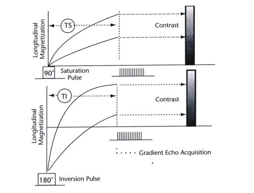
Both SAGE with short TR values and EPI can produce very rapid acquisitions. However, the short time intervals between the gradient echo events do not provide sufficient time for good longitudinal magnetization contrast (T1 or PD) to be formed. This problem is solved by “preparing” the magnetization and forming the contrast just one time at the beginning of the acquisition cycle, as shown in Figure 7-9. Two options are shown.

            The longitudinal magnetization is prepared by applying either a saturation pulse, as in the the inversion-recovery method or an inversion pulse, as in the inversion-recovery method. As the longitudinal magnetization relaxes, contrast is formed between tissues with different T1 and PD values. After a time interval [TI or TS (Time after Saturation)] selected by the operator, a rapid gradient echo acquisition begins.

            The total acquisition time for this method l-is the time required by the acquisition cycles plus the TI or TS time interval.

Mind Map Summary
Gradient Echo Imaging Methods

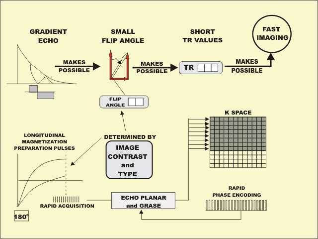
            The common characteristic of the gradient echo imaging methods is that a magnetic field gradient is used to produce the echo event rather than a 180° RF pulse, as is used in the spin echo methods. One of the principal advantages of the gradient echo process is that it is a relatively fast imaging method.

            By using a gradient, and not an RF pulse, to produce the echo event, it is possible to use saturation/excitation pulses with flip angles less than 90˚; thereby all the longitudinal magnetization is not destroyed (saturated) at the beginning of each cycle. Because some longitudinal magnetization carries over from cycle to cycle, it is possible to reduce the TR value and still produce useful signal levels. The reduced TR values result in faster imaging. The flip angle of the RF pulse is an adjustable protocol factor that controls the type of contrast produced.

            Echo planar imaging is a gradient echo method in which many echo events, each with a different phase encoding step, are created during each imaging cycle. This makes it possible to fill multiple rows of k space, which results in very fast imaging. GRASE is an imaging method that combines the principles of echo planar and fast (turbo) spin echo to produce rapid imaging acquisitions.

            When very fast gradient echo methods are used, there is not sufficient time between the echo events for significant tissue relaxation and contrast to develop. Therefore, the desired contrast is developed at the beginning of the acquisition by applying either inversion or saturation “magnetization preparation” pulses. Then, when the desired contrast has developed, a rapid acquisition is performed.